
Continuous Random Variables

Chapter Objectives
By the end of this chapter, the student should be able to:
- Recognize and understand continuous probability density functions in general.
- Recognize the uniform probability distribution and apply it appropriately.
- Recognize the normal probability distribution and apply it appropriately.
- Recognize the standard normal probability distribution and apply it appropriately.
- Compare normal probabilities by converting to the standard normal distribution.
Continuous random variables have many applications. Baseball batting averages, IQ scores, the length of time a long distance telephone call lasts, the amount of money a person carries, the length of time a computer chip lasts, and SAT scores are just a few. The field of reliability depends on a variety of continuous random variables.
Note
The values of discrete and continuous random variables can be ambiguous. For example, if X is equal to the number of miles (to the nearest mile) you drive to work, then X is a discrete random variable. You count the miles. If X is the distance you drive to work, then you measure values of X and X is a continuous random variable. For a second example, if X is equal to the number of books in a backpack, then X is a discrete random variable. If X is the weight of a book, then X is a continuous random variable because weights are measured. How the random variable is defined is very important.
Properties of Continuous Probability Distributions
The graph of a continuous probability distribution is a curve. Probability is represented by area under the curve.
The curve is called the probability density function (abbreviated as pdf). We use the symbol f(x) to represent the curve. f(x) is the function that corresponds to the graph; we use the density function f(x) to draw the graph of the probability distribution.
Area under the curve is given by a different function called the cumulative distribution function (abbreviated as cdf). The cumulative distribution function is used to evaluate probability as area.
- The outcomes are measured, not counted.
- The entire area under the curve and above the x-axis is equal to one.
- Probability is found for intervals of x values rather than for individual x values.
- P(c < x < d) is the probability that the random variable X is in the interval between the values c and d. P(c < x < d) is the area under the curve, above the x-axis, to the right of c and the left of d.
- P(x = c) = 0 The probability that x takes on any single individual value is zero. The area below the curve, above the x-axis, and between x = c and x = c has no width, and therefore no area (area = 0). Since the probability is equal to the area, the probability is also zero.
- P(c < x < d) is the same as P(c ≤ x ≤ d) because probability is equal to area.
We will find the area that represents probability by using geometry, formulas, technology, or probability tables. In general, calculus is needed to find the area under the curve for many probability density functions. When we use formulas to find the area in this textbook, the formulas were found by using the techniques of integral calculus. However, because most students taking this course have not studied calculus, we will not be using calculus in this textbook.
There are many continuous probability distributions. When using a continuous probability distribution to model probability, the distribution used is selected to model and fit the particular situation in the best way.
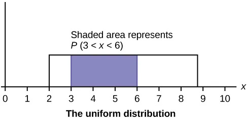
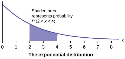
In this chapter and the next, we will study the uniform distribution, the exponential distribution, and the normal distribution. The following graphs illustrate these distributions.
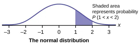
The normal, a continuous distribution, is the most important of all the distributions. It is widely used and even more widely abused. Its graph is bell-shaped. You see the bell curve in almost all disciplines. Some of these include psychology, business, economics, the sciences, nursing, and, of course, mathematics. Some of your instructors may use the normal distribution to help determine your grade. Most IQ scores are normally distributed. Often real-estate prices fit a normal distribution. The normal distribution is extremely important, but it cannot be applied to everything in the real world.
In this chapter, you will study the normal distribution, the standard normal distribution, and applications associated with them.
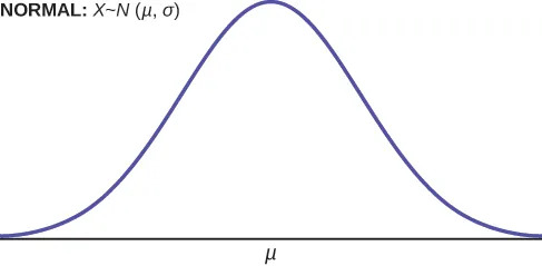
The normal distribution has two parameters (two numerical descriptive measures): the mean (μ) and the standard deviation (σ). If X is a quantity to be measured that has a normal distribution with mean (μ) and standard deviation (σ), we designate this by writing
The probability density function is a rather complicated function. Do not memorize it. It is not necessary.
$$f(x)=\frac{1}{\sigma \cdot \sqrt{2\pi}}\cdot e^{-\frac{1}{2}\cdot \left( \frac{x-\mu}{\sigma} \right)^2}$$
The cumulative distribution function is P(X < x). It is calculated either by a calculator or a computer, or it is looked up in a table. Technology has made the tables virtually obsolete. For that reason, as well as the fact that there are various table formats, we are not including table instructions.
The curve is symmetric about a vertical line drawn through the mean, μ. In theory, the mean is the same as the median, because the graph is symmetric about μ. As the notation indicates, the normal distribution depends only on the mean and the standard deviation. Since the area under the curve must equal one, a change in the standard deviation, σ, causes a change in the shape of the curve; the curve becomes fatter or skinnier depending on σ. A change in μ causes the graph to shift to the left or right. This means there are an infinite number of normal probability distributions. One of special interest is called the standard normal distribution.
