Using the Normal Distribution

jkesler

Continuous Random Variables

24 Using the Normal Distribution

[latexpage]

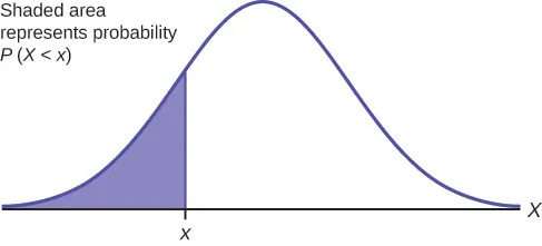
The shaded area in the following graph indicates the area to the left of x. This area is represented by the probability P(X < x). Normal tables, computers, and calculators provide or calculate the probability P(X < x).

This diagram shows a bell-shaped curve with uppercase X at the extreme right end of the X axis. The X axis also contains a lowercase x about one-quarter of the way across the X axis from the right. The area under the bell curve to the right of the lowercase x is shaded. The label states: shaded area represents probability P(X < x).

Figure 6.4

The area to the right is then $P(X>x) = 1 –P(X<x)$. Remember, $P(X<x) =$ Area to the left of the vertical line through $x$. $P(X >x) = 1 –P(X<x) =$ Area to the right of the vertical line through $x$. $P(X<x)$ is the same as $P(X≤x)$ and $P(X>x)$ is the same as $P(X\geq x)$ for continuous distributions.

Calculations of Probabilities

Probabilities are calculated using technology. There are instructions given as necessary for Google Sheets, many of which will work fine in other modern spreadsheet applications as well.

NOTE

To calculate the probability without a spreadsheet program, use the probability tables provided in the appendix.

Example 5.13

If the area to the left is 0.0228, then the area to the right is 1 – 0.0228 = 0.9772.

Try It 5.13

If the area to the left of x is 0.012, then what is the area to the right?

Google Sheets: Standard Normal Distribution

The NORM.S.DIST() function assumes $\mu =0$ and $\sigma=1$ and will give you the probability/area to the left of a z-score that you input into the function. For example, if you type =NORM.S.DIST(2.4), the cell will show the value 0.9918024641 (we generally only need 4 decimal places). This tells us that the probability to the left of $z=2.4$ is 0.9918.

In most situations, the mean will not be 0, and/or the standard deviation will not be 1. In these cases, you can convert the value for which you want the probability (what we sometimes will call the “$x$-value”) into a $z$-score with the standard formula below and plug that $z$-score into the NORM.S.DIST() function.

$$z = \frac{x-\mu}{\sigma}$$

NORM.S.DIST

Returns the value of the standard normal cumulative distribution function for a specified value.

Sample Usage

NORM.S.DIST(2.4)

NORM.S.DIST(A2)

Syntax

NORM.S.DIST(x)

x – The input to the standard normal cumulative distribution function.

Notes

The “standard” normal distribution function is the normal distribution function with mean of 0 and variance (and therefore standard deviation) of 1.

Converting between $z$-scores and $x$-values

We have seen that to convert an $x$-value whose distribution is normal with a mean $\mu$ and a standard deviation $\sigma$, we can use the standard $z$-score formula.

$$z=\frac{x-\mu}{\sigma}$$

We often times need to convert a $z$-score back into an $x$-value. A bit of algebraic manipulation on the $z$-score formula gives us the following formula to convert a $z$-score into an $x$-value. We show this in part 3 of Example 6.8 below.

$$ x = z \cdot \sigma + \mu$$

Example 5.14

The final exam scores in a statistics class were normally distributed with a mean of 63 and a standard deviation of 5.

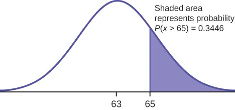
Find the probability that a randomly selected student scored more than 65 on the exam.
Find the probability that a randomly selected student scored less than 85.
Find the 90^th percentile (that is, find the score k that has 90% of the scores below k and 10% of the scores above k).
Find the 70^th percentile (that is, find the score k such that 70% of scores are below k and 30% of the scores are above k).

Solution 5.14

Let X = a score on the final exam. X ~ N(63, 5), where μ = 63 and σ = 5.
Draw a graph.
Then, find P(x > 65) by first converting 65 into a $z$-score.
$z = \frac{x-\mu}{\sigma}=\frac{65-63}{5} = \frac{2}{5} = 0.4$
In a spreadsheet, use the function =NORM.S.DIST(0.4) to find the probability to the left of 0.4 is 0.6554
(Alternatively, lookup the $z$-score 0.4 on the Standard Normal Distribution Table)
Since we want the probability to the right, we take $1-0.6554 = 0.3446$
P(x > 65) = 0.3446

Figure 6.5

The probability that any student selected at random scores more than 65 is 0.3446.

Historical Note

The TI probability program calculates a z-score and then the probability from the z-score. Before technology, the z-score was looked up in a standard normal probability table (because the math involved is too cumbersome) to find the probability. In this example, a standard normal table with area to the left of the z-score was used. You calculate the z-score and look up the area to the left. The probability is the area to the right.
Draw a graph.

Then find P(x < 85), and shade the graph.

Convert 85 to a $z$-score.

$z=\frac{85-63}{5} = 4.4$

Use the spreadsheet function =NORM.S.DIST(4.4) to find the probability to the left of 4.4, P(z < 4.4) = 1.

The probability that one student scores less than 85 is approximately one (or 100%).
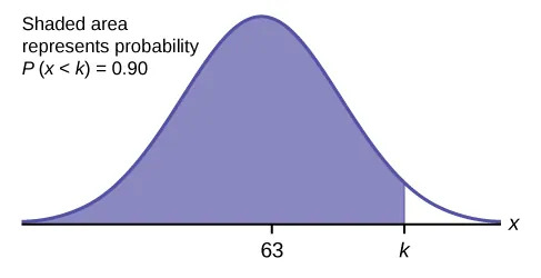
Find the 90^th percentile. For each problem or part of a problem, draw a new graph. Draw the x-axis. Shade the area that corresponds to the 90^th percentile.Let k = the 90^th percentile. The variable k is located on the x-axis. P(x < k) is the area to the left of k. The 90^th percentile k separates the exam scores into those that are the same or lower than k and those that are the same or higher. Ninety percent of the test scores are the same or lower than k, and ten percent are the same or higher. The variable k is often called a critical value.

Figure 6.6

In a spreadsheet, use the function =NORM.S.INV(0.9) to find the $z$-score with 90% of the area to the left. We find it is 1.28 (see below for more information on the NORM.S.INV function)

(Alternatively, find the probability closest to 0.9 on the Standard Normal Distribution Table, and use the associated $z$-score. The closest probability to 0.9 is 0.8997, and its associated $z$-score is 1.28)

Convert $z=1.28$ into an $x$-value given the mean $\mu = 63$ and standard deviation $\sigma = 5$

$x = z\cdot \sigma + \mu = (1.28) 5 + 63 = 69.4 $

The 90^th percentile is 69.4. This means that 90% of the test scores fall at or below 69.4 and 10% fall at or above.
Find the 70^th percentile.

Draw a new graph and label it appropriately. k = 65.6

The 70^th percentile is 65.6. This means that 70% of the test scores fall at or below 65.5 and 30% fall at or above.

invNorm(0.70,63,5) = 65.6

Google Sheets: Inverse Standard Normal Distribution

When we need to take a probability and find the associated $z$-score, we can use the NORM.S.INV() function. Note, this is the reverse of what we did previously with the NORM.S.DIST() function, where we had a $z$-score and we needed to find the probability.

In part 3 of Example 6.8, we used =NORM.S.INV(0.9) to find that 1.28 was the $z$-score that had 0.9, or 90% to the left.

1.28 is then said to be the 90^th percentile.

NORM.S.INV

Returns the value of the inverse standard normal distribution function for a specified value.

Sample Usage

NORM.S.INV(.75)

NORM.S.INV(A2)

Syntax

NORM.S.INV(x)

x – The input to the inverse standard normal distribution function.

Notes

The “standard” normal distribution function is the normal distribution function with mean of 0 and variance (and therefore standard deviation) of 1.
x must be greater than 0 and less than 1 or a #NUM! error will occur.

Try It 5.14

The golf scores for a school team were normally distributed with a mean of 68 and a standard deviation of three.

Find the probability that a randomly selected golfer scored less than 65.

Example 5.15

A personal computer is used for office work at home, research, communication, personal finances, education, entertainment, social networking, and a myriad of other things. Suppose that the average number of hours a household personal computer is used for entertainment is two hours per day. Assume the times for entertainment are normally distributed and the standard deviation for the times is half an hour.

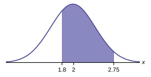
Find the probability that a household personal computer is used for entertainment between 1.8 and 2.75 hours per day.
Find the maximum number of hours per day that the bottom quartile of households uses a personal computer for entertainment.

Solution 5.15

Let X = the amount of time (in hours) a household personal computer is used for entertainment. X ~ N(2, 0.5) where μ = 2 and σ = 0.5.Find P(1.8 < x < 2.75).The probability for which you are looking is the area between x = 1.8 and x = 2.75.

Figure 6.7

Convert 2.75 to a $z$-score.

$z = \frac{x-\mu}{\sigma}=\frac{2.75 – 2}{0.5} =1.5$

Find the probability to the left of 1.5.

=NORM.S.DIST(1.5) gives us 0.9332

Convert 1.8 to a $z$-score

$z = \frac{x-\mu}{\sigma}=\frac{1.8- 2}{0.5} =-0.4$

Find the probability to the left of -0.4

=NORM.S.DIST(-0.4) gives us 0.3446

Subtract the smaller area from the larger area

0.9332 – 0.3446 = 0.5886

Note we could have put both our spreadsheet formulas in one line and had the spreadsheet do the subtraction for us =NORM.S.DIST(1.5)-NORM.S.DIST(-0.4)

The probability that a household personal computer is used between 1.8 and 2.75 hours per day for entertainment is 0.5886.
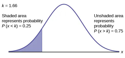
To find the maximum number of hours per day that the bottom quartile of households uses a personal computer for entertainment, find the 25^th percentile, k, where P(x < k) = 0.25.

Figure 6.8

Find the $z$-score with 0.25 to the left

=NORM.S.INV(0.25) to find $z= -0.67$

Convert $z=-0.67$ to an $x$-value

$x = -0.67 ( 0.5) + 2 = 1.66$

The maximum number of hours per day that the bottom quartile of households uses a personal computer for entertainment is 1.66 hours.

Try It 5.15

The golf scores for a school team were normally distributed with a mean of 68 and a standard deviation of three. Find the probability that a golfer scored between 66 and 70.

Example 5.16

In the United States the ages 13 to 55+ of smartphone users approximately follow a normal distribution with approximate mean and standard deviation of 36.9 years and 13.9 years, respectively.

Determine the probability that a random smartphone user in the age range 13 to 55+ is between 23 and 64.7 years old.
Determine the probability that a randomly selected smartphone user in the age range 13 to 55+ is at most 50.8 years old.
Find the 80^th percentile of this distribution, and interpret it in a complete sentence.

Solution 5.16

Convert the ages 23 and 64.7 to $z$-scores, then find the probability between the two $z$-scores
1. $z_{23} = \frac{23-36.9}{13.9}=-1$ and $z_{64.7} = \frac{64.7-36.9}{13.9} = 2$
2. =NORM.S.DIST(2) – NORM.S.DIST(-1) = 0.8186
Convert the age 50.8 to a $z$-score, then find the probability below the $z$-scores
1. $z = \frac{50.8-36.9}{13.9}=1$
2. =NORM.S.DIST(1) = 0.8413
Find the $z$-scores associated with 0.8 to the left, then the $z$-scores to an $x$-value
1. =NORM.S.INV(0.8) = 0.84
2. $x = z\cdot \sigma + \mu = 0.84 (13.9) + 36.9 = 48.6$
3. 80% of the smartphone users in the age range 13 – 55+ are 48.6 years old or less.

Try It 5.16

Use the information in Example 5.16 to answer the following questions.

Find the 30^th percentile, and interpret it in a complete sentence.
What is the probability that the age of a randomly selected smartphone user in the range 13 to 55+ is less than 27 years old.

Example 5.17

In the United States the ages 13 to 55+ of smartphone users approximately follow a normal distribution with approximate mean and standard deviation of 36.9 years and 13.9 years respectively. Using this information, answer the following questions (round answers to one decimal place).

Calculate the interquartile range (IQR).
Forty percent of the smartphone users from 13 to 55+ are at least what age?

Solution 5.17

Recall IQR = Q₃ – Q₁. Find the $z$-scores associated with Q₃ = 75^th percentile and Q₁ = 25^th percentile. Convert the $z$-scores into $x$-values and subtract them.
1. =NORM.S.INV(0.75) = 0.6745 & =NORM.S.INV(0.25) = -0.6745 (note these are opposites, which is not a coincidence)
2. Q₃ = 0.6745 (13.9) + 36.9 = 46.2756 & Q₁ = -0.6745 (13.9) + 36.9 = 27.5245
3. IQR = Q₃ – Q₁ = 18.8
The key words “at least” tell us the 40% is on the right side of the normal distribution, so 60% is on the left. We will convert 0.6 to a $z$-score and convert it to an $x$-value.
1. =NORM.S.INV(0.6) = 0.25
2. $x = 0.25 (13.9) + 36.9 = 40.4$
3. Forty percent of the smartphone users from 13 to 55+ are at least 40.4 years.

Try It 5.17

Two thousand students took an exam. The scores on the exam have an approximate normal distribution with a mean μ = 81 points and standard deviation σ = 15 points.

Calculate the first- and third-quartile scores for this exam.
The middle 50% of the exam scores are between what two values?

Example 5.18

A citrus farmer who grows mandarin oranges finds that the diameters of mandarin oranges harvested on his farm follow a normal distribution with a mean diameter of 5.85 cm and a standard deviation of 0.24 cm.

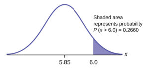
Find the probability that a randomly selected mandarin orange from this farm has a diameter larger than 6.0 cm. Sketch the graph.
The middle 20% of mandarin oranges from this farm have diameters between ______ and ______.
Find the 90^th percentile for the diameters of mandarin oranges, and interpret it in a complete sentence.

Solution 5.18

Convert 6.0 cm to a $z$-score and find the probability to the right of that $z$-score (it is to the right because we are asked about “a diameter larger than 6.0 cm”).
1. $z = \frac{6-5.85}{0.24} = 0.625$
2. =1 – NORM.S.DIST(0.625) = 0.2660 (we subtract from 1 here because we want the probability to the right )
3. Figure 6.9
Note that the middle 20% is between 40% and 60%. Find the $z$-scores associated with 40% and 60%. Convert those $z$-scores into $x$-values (orange diameters in this case)
1. =NORM.S.INV(0.4) =-0.25 & =NORM.S.INV(0.6) = 0.25
2. $x_{40} = -0.25 (0.24) + 5.85 = 5.79$ cm
3. $x_{60} = 0.25 (0.24) + 5.85 = 5.91$ cm
4. The middle 20% of mandarin oranges from this farm have diameters between 5.79 cm and 5.91 cm.
Find the $z$-score associated with 90%, and convert it to an $x$-value
1. =NORM.S.INV(0.9) = 1.28
2. $x = 1.28 (0.24) + 5.85 = 6.16$
3. 90% of the farmer’s mandarin oranges have a diameter smaller than 6.16 cm.

Try It 5.18

Using the information from Example 5.18, answer the following:

The middle 40% of mandarin oranges from this farm are between ______ and ______.
Find the 16^th percentile and interpret it in a complete sentence.

Alternative Spreadsheet Functions

In the calculations we have performed here, we have had to calculate $z$-scores before arriving at an answer. There are two spreadsheet functions analogous to NORM.S.DIST and NORM.S.INV which allow you to bypass the $z$-score calculation. More specifically, these analogous functions perform the $z$-score calculation behind the scenes, but you must provide these functions the distribution mean and standard deviation.

If you would like to learn more about these functions and how to use them, click on the links below:

License

Icon for the Creative Commons Attribution 4.0 International License

Introductory Statistics with Google Sheets by jkesler is licensed under a Creative Commons Attribution 4.0 International License, except where otherwise noted.